
Overview#
svmbir is a Python package for Model Based Iterative Reconstruction (MBIR) of parallel-beam and fan-beam tomography data. It wraps the super-voxel C code sv-mbirct, written by High Performance Imaging and now maintained in this repository, which implements the super-voxel algorithm [A3] [A4] on multi-core CPUs.
Image quality: MBIR uses a forward (sensor) model and a prior (image) model, so it does well on sparse-view and noisy data.
Speed: the super-voxel algorithm is 100 to 1000 times faster than conventional MBIR code, because it reorganizes the computation to match the processor’s cache. Part of this is a precomputed system matrix for the scan geometry, stored on disk and reused whenever the same geometry recurs.
Plug-and-Play priors: a proximal map interface lets any denoiser serve as the prior [A2] [A1].
svmbir is the older CPU package of the OpenMBIR family. New development, GPU reconstruction, and cone-beam, helical, and laminography geometries are in MBIRTorch. See Quick Start for a first reconstruction and Installation to install.
Geometry
svmbir supports the parallel-beam and fan-beam geometries below.
Fan beam has two detector shapes, selected with the geometry argument.
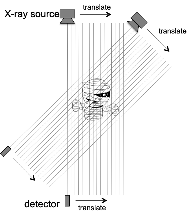
Parallel-beam geometry# |
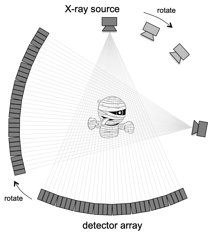
Fan-beam geometry# |
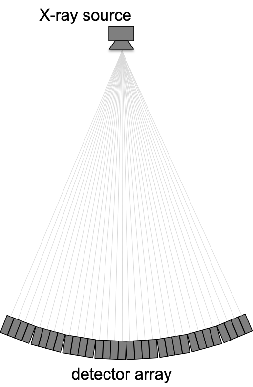
Equiangular (geometry=’fan-curved’)# |
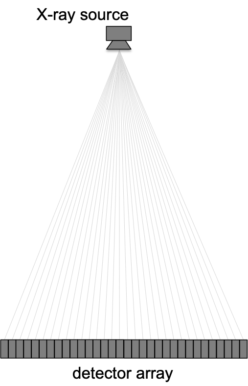
Equal spaced (geometry=’fan-flat’)# |
Note on view angle ordering
In certain imaging systems with slow acquisition, it is common practice to collect view data using techniques such as the “golden ratio” method in which the view angles are not collected in monotonically increasing order on the interval \([0,2\pi)\). While svmbir will produce the correct reconstruction regardless of view ordering, its reconstruction speed will be substantially degraded when the views are not in monotone order. In this case, we highly recommend that users reorder the sinogram views using the provided sino_sort function. The sino_sort function first wraps the view angles modulo \(2\pi\), and then sorts the views to be in monotonically increasing order by view angle.
Conversion from Arbitrary Length Units (ALU)
In order to simplify usage, reconstructions are done using arbitrary length units (ALU). In this system, 1 ALU can correspond to any convenient measure of distance chosen by the user. So for example, it is often convenient to take 1 ALU to be the distance between pixels, which by default is also taken to be the distance between detector channels.
Transmission CT Example: For this example, assume that the physical spacing between detector channels is 5 mm. In order to simplify our calculations, we also use the default detector channel spacing and voxel spacing of delta_channel=1.0 and delta_xy=1.0. In other words, we have adopted the convention that the voxel spacing is 1 ALU = 5 mm, where 1 ALU is now our newly adopted measure of distance.
Using this convention, the 3D reconstruction array, image, will be in units of \(\mbox{ALU}^{-1}\). However, the image can be converted back to more conventional units of \(\mbox{mm}^{-1}\) using the following equation:
Emission CT Example: Once again, we assume that the channel spacing in the detector is 5 mm, and we again adopt the default reconstruction parameters of delta_channel=1.0 and delta_xy=1.0. So we have that 1 ALU = 5 mm.
Using this convention, the 3D array, image, will be in units of photons/AU. However, the image can be again converted to units of photons/mm using the following equation:
Matrix caching
When system matrices are computed, they are stored to disk and will be automatically loaded whenever the same geometry is subsequently encountered.
By default, the system matrices are stored in the subfolder ~/.cache/svmbir/sysmatrix of your home directory.
The matrix files can be removed at any time, and should be periodically cleaned out to reduce disk use.
Occasionally, updates to the software package include changes to the encoding of the system matrix, in which case the the cached matrix files should also be cleaned out to avoid incompatibility.